Module 11 - The end of Class!!! and Toolboxes

This last week in Programming was dedicated to learning how to share toolboxes and script tools for ArcGIS as well as finishing up final projects. Both of these were just the icing on the cake for an awesome class. Not only can I create my own scripts now, I can turn them in to tools and share them with other people who have never used Python before.

I wish I would have learned how to work with Python five years ago and I am excited to continue learning more about it. I will definitely be using Python scripts in the future as I continue to work with ArcGIS and I will be creating tools to share with my coworkers. The most useful thing I learned in this course is how to use a Python script to make large amounts of spatial data more manageable. I can now write and run a script to search the attributes of a point file, select a particular value, and clip that specific data from a 500,000 point file without opening a map. Now I can also string multiple processes together with a script, model, or script tool which will save a ton of time.

The most interesting thing I learned was how simple Python is to use and understand. I wanted to learn how to write scripts for several years but I was afraid of how complex the process would be. I had no knowledge of programming languages before this course other than how confusing they sounded when other people talked about them. I’m not saying Python is super easy because it surely stumped me a few times, but it is not something people should be afraid to try out.

Big Data and Travel Studies - Participation #2

Is more spatial data always better? Is there a point where the quality and details in a dataset can be outweighed by an extremely large amount of data lacking any detail beyond time stamps and coordinates?

The article I chose this week addresses big data and the issue of quantity vs. quality. The study focused on comparing the accuracy identifying individual and household travel activity and behavior between traditional data collection surveys and GPS based surveys. Traditionally this data is collected through surveys where people logged their activity for a one or two day period and sent in their survey response. The information includes where and when people traveled as well as mode of travel and purpose of travel. Voluntary participation and survey costs limit the data that can be collected. GPS based surveys, on the other hand, can easily collect data from hundreds of thousands of people with the acceptance of an application on a smart phone. The time and travel as easily collected with no additional user input but this large amount of data lacks details about method of travel and purpose of travel. This is where Python and spatial analysis come in.

The study used conducted three experiments analyzing GPS based travel surveys on one study using traditional survey data from San Francisco. Each experiment used the same data but a different algorithm to process the data. The San Francisco data was ran through the algorithms as well to compare the results for accuracy. The purpose of the analysis was to try to correctly discern the method of travel and purpose of travel using spatial analysis as well as extra data from accelerometers and Wi-Fi devices contained in phones. Scripts were written using SciPY functions and were applied to the spatial data.

The results showed that big data was useful in identifying patterns in where and when people travel but was not accurate in determining the method of travel or purpose of travel. The smaller the sample size the more accurate the algorithms were but this is the opposite of what is necessary to process big data. If details aren’t necessary for the travel study then big data is a great option, but if purpose and method of travel are needed, study participants will still need to provide information beyond simply carrying their phones.

Title and Link - When is big data big enough? Implications of using GPS-based surveys for travel demand analysis
Or the DOI: doi:10.1016/j.trc.2015.04.025

Module 10 - Creating Custom Tools

This week finishes up Module 10 in GISProgramming which means only one week left! This week the focus was on creating a custom tool in ArcMap based off of an existing stand-alone Python script. I haven't worked on Module 11 yet but I think this might be the most useful part of the course granted this section would not be possible without all of the background knowledge I have now.

For the lab we were given a stand-alone script and the direction for turning it in to a script tool in ArcMap. The script tool we created clipped multiple files to the same boundary area at one time. This is my very general description of how to create a script tool:

Multi-Clip Script Tool

1.       Create stand-alone Python script that performs geoprocessing within ArcMap. 

2.       In ArcMap create new Toolbox in the desired folder in the Catalog window (the same folder the script is saved in).

3.       Add a new script tool to the new Toolbox. This will open the new script tool window.

4.       Set the name, description, store relative paths option, and file path to the stand-alone script in the new script tool window.

Script Tool messages printed to the Results window in ArcMap

5.       Set tool parameters for the script tool either in the script tool wizard or in the script tool properties.

6.       Edit the stand-alone script to reflect the tool parameters set for the script tool instead of absolute paths with the arcpy.GetParameter() code.

7.       Within the stand-alone script change print statement to arpy.AddMessage() statements so the messages will print in the Results window in ArcMap.

By setting the parameters, in both the tool and the original script, you can turn a script that processes on set of data into a tool that can run a particular process on lots of different data (as long as it is the same data type).Knowing how to build these tools would have made GIS Applications labs a little easier and quicker to work through.



-A note for the final project-
I forgot to add updates about my final project the last few weeks. I decided to work with a large .csv containing crime data points that I downloaded from the San Diego Regional Data Warehouse for my Applications class. There was way too much data to work with in ArcMap initially so I wrote a script to display to the points, save the points as a feature class, clip to points to a particular buffer zone, and then separate the points by year. I presented the script project this week in GISProgramming and I'll be working with the data this weekend to finish my analysis project for Application.

Module 9 - Working with Rasters

In Programming this week the focus was solely on working with rasters and the Spatial Analyst module available in arcpy (arcpy.sa). For the lab this week the task was to write a script to find areas that met certain criteria in two separate rasters and combine those areas in to one raster showing only two values, areas meeting all criteria and other areas. As I wrote that last statement it seemed like a very easy, but possibly time consuming, task to complete since I've done done this a few times in my Applications class this semester just using the tools in ArcToolbox. The challenging and time saving part to that statement is all of the work was done with a Python script and barely touched ArcMap to complete all of it. One of the most important parts of working with rasters in a spatial analyst sense is having the license for the Spatial Analyst Extension and having the extension enabled in ArcMap. Without those two things, all of the raster manipulating I did this week would not have been possible.

As for the lab, it started with working with a landcover raster. For this raster I selected all three categories of forests in teh landcover types and used the RemapValue to list them along with the new values I wanted to give them. Then I used the Reclassify tool to reclassify the landcover raster based on those new values. The second raster I worked with was an elevation raster. I used the Slope and Aspect tools to create two temporary rasters based on the original elevation raster. These temporary rasters were used to create four more temporary rasters marking the high and low limits for the slope and aspect criteria. Using map algebra I combined the high and low limits as well as the reclassified forest raster with the "&" (and) character to create the final raster shown below. Finally I used the save method to permanently save only this last file. The final raster contains only two values to identify areas that do or do not meet all of the required criteria.

Raster showing areas meeting slope, aspect, and landcover criteria

Module 8 - Working with Geometries

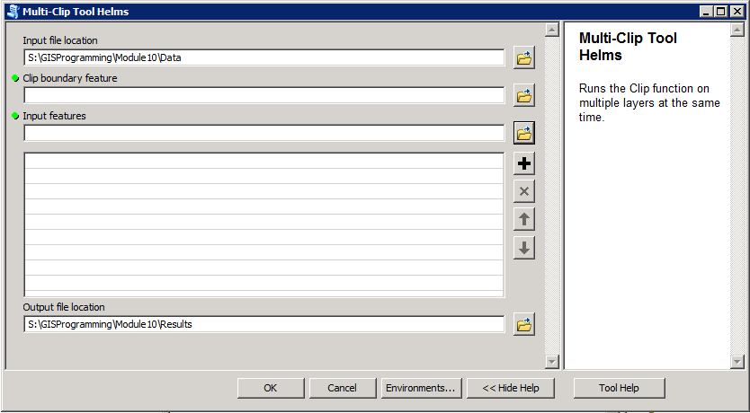
The lab tasks in GIS Programming are getting a little more complicated but completing them definitely feels more rewarding. This week's assignment was to take an existing line shapefile and write a script that captures the geometry for each line segment then writes the data to a new text file. The text file needed to include five items for each vertex in the river shapefile: the OID, the vertex ID, the x-coordinate, the y-coordinate, and the river name. I used PythonWin to write the script and verified my results by viewing the original shapefile in ArcMap. 

Here is the psuedocode for the script I wrote:

§-  Import arcpy module

§ - enable geoprocessing environment file overwriting

§ - set workspace environment/file location to Module8/Data folder

§ - create variable for rivers.shp

§ - search rivers.shp for data using cursor search to find OID, XY coordinates, and river names

§ - create blank text document called rivers.txt and save in Module8/Results folder

§ - use for loop to iterate search through rivers.shp to find row information

-   add variable named vertID to identify the number of parts/vertices in each river

-   use for loop to iterate search through each row to find information about parts/vertices

-  add 1 to vertID variable to count the number of parts in each river

-  use write function to write data line for each stream part to the rivers.txt file (data line consists of OID, vertex number, X coordinate, Y coordinate, river name), include “\n” to separate each line. Note the data line elements are numbered in the order they are listed in the cursor search from earlier, ex. OID = 0

- print data line to verify script progress

§ - close write function

§ - delete row

§ - delete cursor

§  -------

§ - open rivers.txt to verify file was created and data was populated

While writing this script I got stumped two times. The first time was with creating the search cursor to sift through the original shapefile. I could not figure out the proper formatting for the different fields I wanted the search to return. After searching through the textbook and ArcMap's Help Menu I realized the issue was with my spacing and use of brackets/quotations. The next issue took me a lot longer to figure out but was even more simple than the first. I could not figure out how to add a vertex count to my second for loop. I mean I could not figure out how to use the variable I created to increase by one for each part that the loop parsed through. The key to that issue was following the directions and setting the vertex variable to zero in the first loop and then adding one to the variable in the second nested loop. I did a lot of experimenting with that section before the directions and my trials and errors finally clicked in my head.

The results of my script are in the screen capture below. The left column is the OID number (line number) from the shapefile. The second column is the vertex ID that I added within the nested for loops that added a count of vertices in each line. The third and fourth columns list the x and y

coordinates respectively. The last column lists the river name from the shapefile.

Geometries of rivers.shp in a text file

Lab 8 - Damage Assessments

The last lab! This week finished up the last lab in GIS Applications and the focus was on conducting damage assessments after natural disasters using a GIS. Our readings for the week primarily covered water based natural disasters like tsunamis and hurricanes but I think some of the tools used could be applied to other things like earthquakes and tornadoes too. Hurricane Sandy was the topic for the final lab with an in depth look at several blocks in a  town in New Jersey. We used pre-event and post-event images to assess the damage in a three block study area in ArcMap. The first step was to set up a geodatabase and populate it with the different features that would be useful in conducting a damage assessment like county boundaries, property lines, and raster image mosiacs. Once all of the data was set up I moved on to the analysis.

I created a new point feature class to annotate the damage to buildings in the study area. The first thing I did was add one point to each land parcel each using the pre-storm imagery as a reference. I accidentally added multiple points on a few parcels when I first started as I went back and forth between attributes and creating features so I decided to add all of the points first. Then to identify the damage I zoomed in to 1/3 of a block at a time and used the Flicker Tool on the Effects Toolbar to go back and forth between pre and post storm imagery. (The Flicker Tool is great and i wish knew about it sooner. The tool lets you lift up the top layer and look beneath it without having to wait for the whole image to reload, almost like lifting the corner of a newspaper to look at the next page.) Some of the damage was very easy to identify and categorize because the buildings were completely gone but other areas were more difficult. 

Post-event image of study area with structure damage categories, original coastline and 100m, 200m, and 300m markers

From looking at the study area as a whole and then looking at the zoomed in view there appeared to be sand covering everything that was previously pavement or grass. Due to the sand movement I considered every parcel inundated and every structure at least “Affected”. Shadows made it difficult to discern how much damage occurred on some parcels so I looked at the surrounding properties to help estimate the amount of damage. I could not tell if all of the displaced items and buildings moved due to water flow or wind so I also considered every parcel with a vertical structure at least “Affected” by wind if not worse.  Buildings with roof damage were given a higher wind damage rating. Buildings that were completely destroyed were only given a wind rating of “Affected”. Wind damage was the most difficult category to evaluate. 

My results for the three block study area are in the table below.

Structural Damage Category	Count of Structures Within Distance Categories from Coastline
	0-100m	100-200m	200-300m
No Damage	0	0	0
Affected	4	0	5
Minor Damage	0	2	20
Major Damage	1	28	21
Destroyed	7	10	0
Total	12	40	46